
Introduction
Geospatial analysis often involves understanding the spatial relationships between data points. One foundational concept in this domain is the variogram. In this article, we will explore what a variogram is, how it is used in Kriging, and how to compute experimental and semi-variograms for hypothetical borehole data. Finally, we will use these concepts to interpolate water levels across all data points using Kriging.
A Note on Spatial Relationships
The First Law of Geography, proposed by Waldo Tobler, states:
“Everything is related to everything else, but near things are more related than distant things.”
This principle forms the backbone of variogram analysis and Kriging.
What is a Variogram?
A variogram is a graphical representation or function that quantifies the spatial autocorrelation of a dataset. It demonstrates how similarity between measurements decreases with increasing distance.
Key Components of a Variogram
- Lag Distance (h): The separation distance between data points.
- Semivariance (γ(h)): A measure of the dissimilarity between data points separated by distance
h. - Sill: The semivariance value where the variogram levels off, representing the data’s overall variance.
- Range: The distance at which the variogram reaches the sill, indicating the limit of spatial correlation.
- Nugget: The y-intercept of the variogram, accounting for measurement errors or microscale variations.
Variogram Models
Variogram models are mathematical functions used to fit experimental variograms. These models capture the spatial dependence of the data and are essential for Kriging. Commonly used models include:
- Spherical Model:
- Formula: \[ \gamma(h) = \begin{cases} C_0 + C \left[\frac{3h}{2a} - \frac{h^3}{2a^3}\right], & 0 \leq h \leq a \\ C_0 + C, & h > a \end{cases} \]
- Characteristics:
- Commonly used in geosciences.
- Levels off at the range (
a). - Represents a gradual transition of spatial correlation.
- Exponential Model:
- Formula: \[ \gamma(h) = C_0 + C \left(1 - e^{-h/a}\right) \]
- Characteristics:
- Suitable for phenomena with continuous but less abrupt changes.
- Correlation decreases exponentially with distance.
- Gaussian Model:
- Formula: \[ \gamma(h) = C_0 + C \left(1 - e^{-\left(\frac{h}{a}\right)^2}\right) \]
- Characteristics:
- Smooth transitions, often used in environmental studies.
- Effective for data with strong local correlations.
- Linear Model:
- Formula: \[ \gamma(h) = C_0 + C h \]
- Characteristics:
- Represents a direct, proportional increase in semivariance with distance.
- Simplistic but useful for certain datasets.
- Power Model:
- Formula: \[ \gamma(h) = C_0 + C h^k, \quad 0 < k < 2 \]
- Characteristics:
- Flexible model for datasets with non-linear spatial relationships.
Each model serves specific purposes based on the dataset and the spatial behavior being analyzed. Selecting the appropriate variogram model is crucial for accurate Kriging.
The summary of selecting a variogram model presented below:
| Condition | Recommended Model |
|---|---|
| Sharp cutoff in spatial correlation | Spherical (Sph) |
| Rapid decay of correlation | Exponential (Exp) |
| Smooth transitions over space | Gaussian (Gau) |
| Flexible/Intermediate behavior | Matérn (Mat) |
| Short-range dominance | Exponential or Matérn |
| Long-range dominance | Spherical or Gaussian |
| Uncertainty about smoothness | Matérn (adjust \(\nu\)) |
Computing the Variogram in R
Here, we demonstrate how to compute an experimental variogram and fit a theoretical model using hypothetical borehole data.
# Generate hypothetical borehole data
set.seed(123)
location <- data.frame(
  x = runif(20, 0, 100),
  y = runif(20, 0, 100)
)
location$water_level <- 50 + rnorm(20, mean = 0, sd = 5)

# View the data
head(location)
## x y water_level
## 1 28.75775 88.95393 44.66088
## 2 78.83051 69.28034 48.91013
## 3 40.89769 64.05068 44.86998
## 4 88.30174 99.42698 46.35554
## 5 94.04673 65.57058 46.87480
## 6 4.55565 70.85305 41.56653Experimental Variogram
if (!require(sp)) { install.packages('sp'); library(sp)}
if (!require(gstat)) { install.packages('gstat'); library(gstat)}

# Convert to spatial object
coordinates(location) <- ~x + y

# Compute experimental variogram
variogram_exp <- variogram(water_level ~ 1, location)
head(variogram_exp)
## np dist gamma dir.hor dir.ver id
## 1 2 7.912548 12.129825 0 0 var1
## 2 2 11.366795 9.534399 0 0 var1
## 3 2 14.046246 17.299652 0 0 var1
## 4 6 15.922439 23.613955 0 0 var1
## 5 4 19.786952 31.321265 0 0 var1
## 6 5 22.195585 18.261615 0 0 var1The formula used above have format independent_variable ~ 1 or independent_variable ~ x+y. X or/and Y, any independent variables or covariates (if applicable). If the formula is ~ 1, it means there are no covariates, and the variogram will be calculated solely based on spatial relationships. The output of variogram_exp is has field such as np, dist, gamma etc…
- np: the number of point pairs for this estimate; in case of a variogramCloud see below
- dist: the average distance of all point pairs considered for this estimate
- gamma: the actual sample variogram estimate
- dir.hor: the horizontal direction
- dir.ver: the vertical direction
- id: the combined id pair
for more information, read the help of gstat::variogram help page in R.
Semivariance Calculation
Experimental variogram will be created with Semivariance against distance. Process is explained is, first, the semivariance \(\gamma(h)\) is computed for each distance bin \(h\). The formula is:
\[ \gamma(h) = \frac{1}{2N(h)} \sum_{i=1}^{N(h)} \left( z(x_i) - z(x_i + h) \right)^2 \]
Where:
- \(N(h)\): Number of point pairs in the distance bin \(h\).
- \(z(x_i)\): Observed value at location \(x_i\).
- \(z(x_i + h)\): Observed value at location \(x_i + h\).
This gives the average squared difference of observed values separated by \(h\).
The formula shown is for computing semivariance for a given lag or distance ℎ, but it is not directly tied to a specific variogram model such as spherical, exponential, or Gaussian. This formula is a general expression used to calculate experimental semivariance, which is then plotted as an experimental variogram Once the experimental variogram is computed, you can fit it with a specific theoretical variogram model, such as Spherical, Exponential, Gaussian, etc. To identify the specific model, you would calculate the semivariances using the given formula, plot them against distance h, and then choose the model that best fits the curve.
There is a very nice youtube video by YT@MiningGeologist explaing the computation semivariance using the above equation.
plot(variogram_exp, main = "Experimental Variogram")
Fitting a Theoretical Model
This involves selecting a mathematical function (e.g., spherical, exponential, Gaussian) to approximate the experimental variogram. The goal is to create a theoretical variogram that can be used in kriging or other geostatistical methods. The output is a smooth, continuous variogram model that represents the spatial variability of the data.
# Fit a variogram model
variogram_model <- fit.variogram(variogram_exp, model = vgm("Sph", range = 50, nugget = 2))

# Plot the fitted model
plot(variogram_exp, variogram_model, main = "Fitted Variogram Model (Spherical)")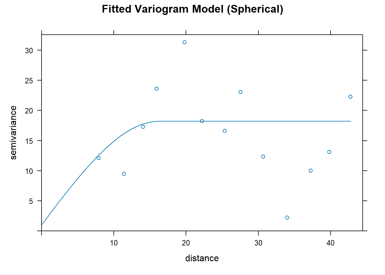
Trying Another Model
# Fit a variogram model
variogram_model_exp <- fit.variogram(variogram_exp, model = vgm("Exp", nugget = 2))

# Plot the fitted model
plot(variogram_exp, variogram_model_exp, main = "Fitted Variogram Model (Exponential)")
Performing Kriging
Once we have a fitted variogram model, we can perform Kriging to interpolate water levels.
# Generate a grid for interpolation
grid <- expand.grid(
  x = seq(0, 100, by = 1),
  y = seq(0, 100, by = 1)
)
coordinates(grid) <- ~x + y

gridded(grid) <- TRUE

# Perform Kriging
kriging_result <- krige(water_level ~ 1, location, grid, model = variogram_model)
## [using ordinary kriging]# Visualize the results
spplot(kriging_result["var1.pred"], main = "Kriging Interpolation")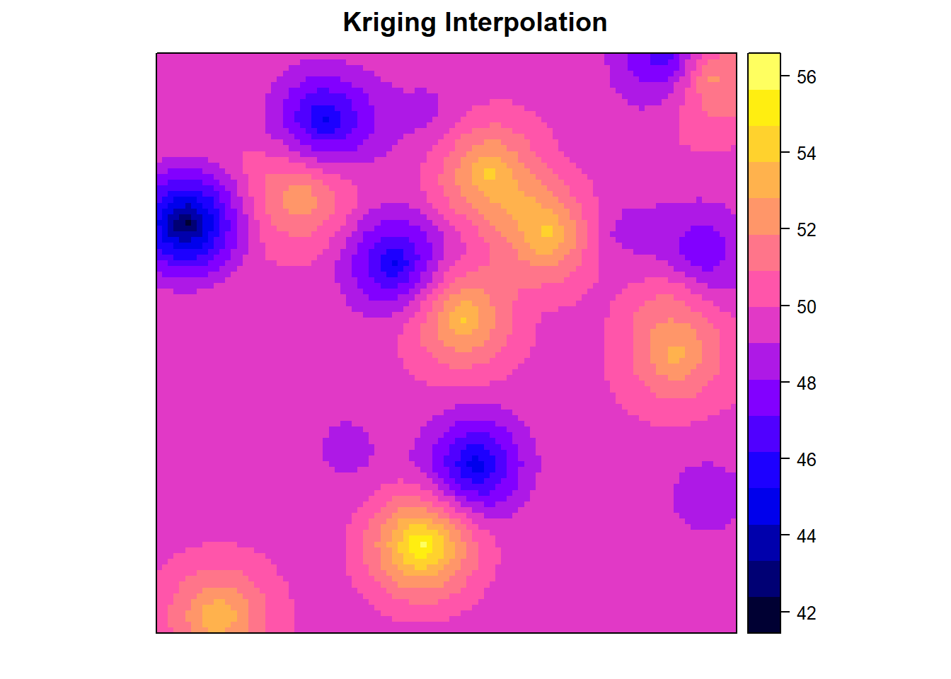
Conclusion
Variograms are an essential tool in geospatial analysis, providing insights into spatial relationships and guiding interpolation techniques. By understanding and applying variogram concepts, we can make informed decisions in various fields, including hydrology, agriculture, and environmental monitoring.